
Instructions
The lead tracker is designed to help you track your progress, diagnose your weaknesses, brag to your friends, get feedback from the community, and conveniently store/manage your growing list of contacts. However, the tracker is only as useful as the information that you provide it, so it's important to understand how that process works. That's why we created this page to walk you through the process of recording your leads and help you get the most out of all the lead tracker's features.
Getting Started
When you first open the lead tracker, you'll only have a few options. As you track more leads and get used to things, you'll unlock more features. For now, let's just focus on what's available: Name, Description, Contact Info, and Notes.
- Name: Name of the person you talked to. If you don't remember or didn't find out, it's okay to leave this blank.
- Description: A short description to help you remember the lead. This description will be combined with the name to create the lead title, which will be used to reference this lead later in the map, history table, etc. It's okay to leave the description blank if this lead is unimportant (i.e., you didn't get their contact info and probably won't see them again).
- Contact Info: Press the pencil button to bring up the contact editor and store/edit their Instagram and/or phone number. Once entered, the main contact buttons on the lead tracker will light up, indicating you can press them to either go to their Instagram page or their text messages (only supported on phones).
- Notes: Put anything else here that you think you'll want to remember later. Can be very useful to use your phone's speech-to-text feature here to quickly record your thoughts and details about your conversation. Makes it much easier to come up with recall humor a day later, especially if you talked to many other leads in the meantime.
Location and Time Auto-Tracking
Don't worry about tracking your time and location. The lead tracker captures this information automatically from your device. After more leads, you'll unlock the ability to view and edit this information via the calendar and map, respectively.
Your First Lead
We'll walk you through how to input your first lead just to show you how simple it is. We'll assume you just did the lead and are using your phone. This process will depend on whether you got their contact info or not...
- No Contact Info: Womp, womp. Better luck next time. The good news though is that you just need to press the big green Create button on the top :)
- Got Contact Info: Nice. If you got their phone number, then press the search button to the right of the name field (or press the blank phone button) to import their name and number directly from your phone's contacts. If you got their Instagram instead, then you'll have to enter this manually instead using the edit button (we'll support Instagram auto-import in the future). Next, write a short description like "Blue suit near fountain" or "Elderly couple with dog". Finally, record any notes about them or your conversation, and press the big green Create button.
That's it! You just recorded your first lead! Super simple stuff.
To see any of these instructions again, just click on Instructions in the top menu.
Lead History Table
Of course, logging leads would be pointless if there were no way to see that data afterwards. The lead history table lets you see important details from all your past leads in a single table. It's a great tool to keep track of which leads you should be paying attention to and which you should move on from. In a future release, you'll be able to customize what columns are shown and how the leads are sorted. You can also click on any row to highlight/select the lead if you want to...
Editing Existing Leads
Enter into Edit mode by selecting a lead from the history table or the map. In Edit mode, the usual new-lead input area is replaced with data from the selected lead, and the Create button on top is replaced with 3 other buttons: Cancel, Update, Delete:
- Cancel: Deselects any selected leads and brings you back to the standard new-lead input area.
- Update: Press the update button after you've made changes in the editor and want to permanently save them. Unsaved changes are highlighted in yellow until you save them. You can view/edit other leads while you have unsaved changes, which are temporarily stored by your local webpage and are indicated by the yellow highlighting of the lead in the history table.
- Delete: Deletes the selected lead.
Map
The map serves several purposes including manually inputting the location of a new lead, editing a previous lead location, or conveniently showing past lead locations.
Marker Colors
To make the map easier to read, different color markers are used for different purposes.
- Red: Old leads. Try to cover the map with these.
- Blue: Your current location. Updated by your device's GPS every few seconds (only works when webpage is open). Note: you might not be able to see this at first because it's usually covered by the...
- Green: New lead. Automatically tracks your current location (blue marker) until you manually move it or until the you start inputting new-lead data causing desynchronization.
- Yellow: Updated lead location. Similar to the green marker, but indicates you're updating the location of a previously recorded lead.
- Orange: Selected lead. Tracks the original unchanged location of the selected lead. As with the blue marker, you might not see this at first while it's covered by the yellow marker.
Editing Leads
Similar to the history table, you can click on any old lead (red marker) to show its title and select it. You can then view and edit the lead as usual.
Auto-Tracking
The auto-track button (bottom-left of map) enters/exits Auto-Track mode. While auto-tracking, the map automatically centers on either the orange selected-location marker or green new-location marker (depending on whether you're in Edit or Input mode, respectively). Manually, moving the map (panning or zooming) will exit Auto-Track mode as well.
Progress
Your progress measures the level of investment from a lead. We've identified 9 levels of progress that are typical milestones of increasing investment. Although it's possible to skip some of these progress milestones, a higher level progress will always indicate more investment than a lower level. We also assume that your progress with a lead is monotonically increasing, meaning you can never regress once you've reached a certain level of investment.
Under these assumptions, the progress model is a powerful yet simple tool for tracking your ability to escalate with leads and identifying your weak points. Although the progress model is simple, it is still important that you feed the model correct data about your real-world progress, so read the following list to understand when you should declare victory on these 9 progress milestones.
- Approached: You got the attention of a potential lead.
- Conversed: You got them to stop (if they were walking) and talk to you. For example, if they stop walking, hear you start talking, and then say "Sorry, I'm not interested" and walks away, that's still Conversed because you got them to stop. This distinction between Approached and Conversed helps us to measure if you need to work on simply approaching/stopping leads. Alternatively, if they're sitting down, you deliver your line, and they pretty much immediately get up and mutter something like "no thanks", then that's also not Conversed.
- Got Contact Info: They gave you their phone number or some kind of social-media contact like Instagram.
- Responded: They either responded to your initial text or texted you first. Texts that occurred during the first meet don't count (e.g., they text you "hi" after getting your number so that you'll have their contact)
- Agreed To Hang: You both agreed to meet at a specific time and place.
- Hung Out: You met each other again. Alternatively, you went on an insta-hang (i.e., went for coffee, snack, drinks while still on the initial meeting).
- Verbal Contract: The lead agreed to purchase your product.
- Purchase Order: You actually received a purchase order.
- Recurring Order: You received a second purchase order on a separate occasion. Doesn't count if they send 2 purchase orders back to back. It may seem strange to claim that the orders are recurring after only the 2nd time, but this is an important separate milestone. Getting to this level means the lead has tried your product, liked it, wants more, and will probably be an ongoing customer into the future.
Status
Unlike progress, which summarizes the lead's history of increasing investment, status represents a current snapshot of where you stand with the lead, which can flip-flop back and forth between hot and cold. In future releases, we will provide the ability to analyze statistics and likelihoods of transitioning from one state to another, but for now, tracking status is still useful as a means for keeping track of which leads you should be paying attention to. From worst to best, the 4 status options are Dead, Left On Read, Ice Ice Baby, I'll Be Back, Top of Mind, and Alive:
- Dead: You'll almost certainly never talk to them again. The most common scenario for Dead is when you were unable to get their contact info during your lead, which makes it pretty hard to continue communications. A less frequent scenario is that their last text said "Leave me alone loser". It's not critical that you be entirely accurate here. If 10% of your "dead" leads come back at some later date, then your status statistics will simply show this to be the case and we'll all know that you're just a little pessimistic.
- Left On Read: You texted them last, and it seems like they probably won't respond back. Because you're not an idiot, you're not going to double text them at this point either. Maybe they'll come back at some point in the future.
- Ice Ice Baby: Similar to Left On Read, but they're the one to text last. Yep. they should have shown more interest, maybe been a little more enthusiastic. You could tell the conversation wasn't going anywhere productive for now, so you left them on read and are now icing them.
- I'll Be Back: There was potential, but you didn't have enough time to progress much before one of you had to leave town. You don't feel like texting to stay top-of-mind, but you'll hit them up when you visit their area again.
- Top of Mind: Things are going well, but you can't make progress right now for logistical reasons. Better text them every 1 to 2 weeks to stay top-of-mind so they don't forget about you.
- Alive: You guys are in relatively consistent communication. Things are progressing normally.
Progress Analysis
You can see various breakdowns of your progress stats in the analysis section of the lead tracker using the 3 different views:
- Highest: Shows the highest level that your leads have progressed to. Because progress can only increase, your highest level is also your current level, so you can think of this view as being a breakdown of your current progress levels. For example, a 50% Highest rating for Conversed means that half of your leads currently have Conversed listed as their progress level. This view can be shown as a raw count or as a percentage of all leads.
- Reached: Shows how often you are able to reach a certain progress level. For example, a 10% Reached rating for Responded means that 10% of your leads at least got to the point where the lead texted you, and possibly further than that. As with Highest, this view can also be shown as a raw count or as a percentage of all leads.
- Skill: Shows your skill at achieving certain progress milestones assuming you already completed the previous milestone. This chart is extremely helpful because it helps isolate analysis of different skills from each other, so you can pinpoint where your actual weaknesses and strengths are. For example, if you only reach Verbal Contract 1% of the time, the Skill view can help you determine if this is because you struggle with getting them to respond to your texts, getting them to meet up again, or just getting them to stop and talk with you in the first place.
Par
A par rating exists in each progress analysis view to show the expected results of someone that has mastered the lead/escalation process. These ratings are based on years of cumulative experience, and are mostly reflective of direct results (we will include non-direct ratings in the future). Knowing par helps users to set realistic expectations for themselves and to identify where they are actually having trouble. For example, it'd be silly to expect to receive purchase orders from 1 out of every 5 leads you meet, and you shouldn't be troubled if your skill at getting leads to text you back is lower than your ability to get a verbal contract while hanging out.
Note: The par line sets a clear goal for the Skill and Reached views since higher values are always better. However, this is not the case for the Highest view, where an excessively high value for a certain level likely indicates that you have trouble passing that level and keep getting stuck there.
Calculation Method
For those who are curious, we describe here how we use the raw lead data to calculate the results shown in the views.
We'll start with the Highest measure, since this is the most straightforward. As stated above, this is simply the count of all leads with a certain progress level. We'll represent this dataset as \(H[n]\), where \(n\) is an integer from 1 to 9 corresponding to one of the 9 progress levels in order from Approached to Recurring Order.
For the Reached dataset \(R[n]\), we count every lead at a certain progress level or above, so...\[ R[n]=\sum_{i=n}^{\infty}H[i] \]
Finally, the Skill dataset \(S[n]\) represents the conditional probability that a certain level is reached given that the previous level was reached. Therefore...\[ S[n]=\frac{R[n]}{R[n-1]} \]
Calendar and Time Editing
Sometimes you might forget to record a lead in the moment or you just might want to do it later. The time auto-tracker will obviously select the incorrect time, so you'll need to manually set the lead time yourself. You can view and edit the currently selected time via the Time input field.
The small text just to the right of the time field shows the current timezone. Clicking on this text will show a popup with more description on the shown timezone. By default, your local timezone is showing, but this won't necessarily be the case when you unlock different timezone modes, so this text can be a helpful reminder of what you're actually looking at in the time field.
Note: The time resolution is limited to minutes.
Timezone Modes
Dealing with timezones can get confusing, but it's a necessary evil when tracking your leads as you travel around the world. Fortunately, we provide 3 timezone modes to help you manage this timezone madness in an intuitive way:
- UTC: You're a hard man of science. You measure temperature in Kelvin, lament that duodecimal will probably never catch on, and you sure-as-shit don't respect the arbitrary man-made nuances of timezones. If this describes you, then Coordinated Universal Time (UTC) is for you. One timezone to rule them all. All times are always the same no matter where you currently are or where the lead occurred.
- Local: Basically what it sounds like. The simplest timezone mode. Just shows the local time wherever you are. This is the default timezone mode until you change it. Note that the lead tracker will detect if your local timezone changes (either by traveling or messing with your device settings), which can abruptly cause a variety of small changes (e.g., displayed times, sort order, timeline data, filter results).
- Approach: If you're collecting and viewing/analyzing leads from around the world, you probably want to use this mode. Instead of showing the timezone where you currently are, this shows the timezone where you first approached the lead. If there's no selected lead, then it'll show the timezone of the new lead you're about to enter (green marker on map), which should be your local timezone. So if you approach a lead at 4pm in New York, and you are now in California, the Local mode would show it at 1pm ET, but the Approach mode will conveniently always recognize it as 4pm ET no matter where you are. Note that Approach time shows the current time at the lead location and does not factor in whether daylight savings was in effect when the lead occurred. This means the approach time can seem to vary by an hour over the course of a year as the corresponding timezone goes in and out of daylight-savings time. Solving this problem well requires knowledge of evolving local laws and their history, and so is beyond the scope of this tool.
Timeline Analysis
Users can use the timeline analysis chart in the analysis section of the lead tracker to see how often and when they've been approaching new leads. Just like with the map, you can pan and zoom with the mouse by dragging the cursor or rolling the scroll wheel, respectively, or via touch by swiping and pinching. The timing resolution can be set to hours, days, weeks, months, or years. In order to level out temporary bumps/spikes and see trends across several units of time, we've provided a gaussian smoothing option which you can set to one of three settings:
- No Smoothing: No smoothing is applied
- Bit Smooth: Gaussian smoothing with a standard deviation of 1.5 time units
- Smoothie: Gaussian smoothing with a standard deviation of 5 time units
On-1st-Meet Events
Sometimes it's possible to escalate really far with a lead even while still on the initial lead. We wanted a way for users to recognize these unique wins and also analyze the effects of these events in aggregate at a later date after approaching enough leads. There are currently 5 different on-1st-meet events that can be recorded:
- On-1st-Meet IG: This may seem redundant with the Instagram-contact field already described above, but it is possible to get one type of contact on the first meeting and get other forms afterward. Including this as an on-1st-meet event lets us record if you collected social media contact during the first meeting or after.
- On-1st-Meet Number: Similar to the on-1st-meet IG event, this input helps distinguish if you got their phone number on the first meeting or afterward.
- Insta-Hang: The most common on-1st-meet event (ignoring the trivial Instagram and phone number events). It takes skill to accomplish this, and it's also a great way to increase the likelihood of seeing the lead again. Doesn't have to be anything fancy. Just a quick sit-down for coffee or drinks.
- Insta-Verbal: You got a verbal confirmation before you parted ways.
- Insta-Order: You silver-tongue seller you. Nice.
Note: It should go without saying that none of these apply to meeting leads online. On-1st-meet events occur from the moment you two became aware of each other until you physically leave each other's presence. Since you're not physically around the leads when you "meet" them online, there is no on-1st-meet period of time.
Viewing Other Users' Leads
You can view other users' leads by going the general-settings area and selecting the desired user you wish to view. This will bring up a similar looking page as your own, except all of the leads will belong to the other user. Use the history table or map to select any of their old leads to view in the lead-input area.
While viewing other users' leads you are locked into Read-Only mode, which provides almost all the same capabilities/tools as the other modes (i.e., input and edit) but with some restrictions. Obviously you can't create new leads, update old leads, or delete them. You also can't see the contact info or notes of their leads because we want our users to feel safe inputting this potentially sensitive info. Finally, you won't be able to see any of the leads that the user has explicitly marked private, which is a feature you can learn more about in the Management Settings section.
Other Inputs
The input fields described here are less important than the others, but some users may still find them useful.
Location Descriptor Input
The lead tracker automatically captures your location's coordinates. This information is easy to show in the map, but is difficult to convey in the table with all the other lead data. Instead, you can write a short location description in the Location text-input field. Use this also to tag different areas with a similar label when appropriate. For example, you might want to use the description "Starbucks" regardless of which particular Starbucks location you're in. Or if a particular street is really good for foot traffic, anywhere along that street could go under that same street name.
Group Size Input
Often, approaching leads in larger groups can be more intimidating, require different strategies, and ultimately be more rewarding. At first, users may want to document group size so they can simply record their accomplishments, but after collecting enough data, they may see encouraging trends indicating that larger groups often result in better outcomes.
Age Input
It can be useful to store the lead's age once they tells you so you can recall it later if necessary. However, it can also be useful to guess the age of every lead you approach so that you can start identifying trends based on their perceived ages. For example, maybe you're more likely to get Instagram from leads who you guess are in their young 20s, but more likely to get recurring orders from older leads in their 50s. This can help you tailor your approach/expectations before you even say hi.
Data Management Settings
Data management settings don't record direct information about the lead. Rather, they record meta-data about how you want to store, use, and share the lead data.
Private
Keep your lead private by activating the button that looks like a vault. Private leads can't be seen by other users, don't count towards competitive events with other users, and don't affect stats that you share with other users. Private leads still appear as normal on your personal lead page and still count normally to your personal stats (e.g., when viewing timeline or progress analysis). In general, we encourage users to use this option sparingly since sharing with the community helps everyone and the most sensitive fields (i.e., notes and contact info) are already hidden regardless.
Do Not Track
Activate Do Not Track mode using the button that looks like a heartbeat covered by the "not allowed" symbol. Untracked leads do not affect your stats (personal or shared) and don't count towards competitive events. Unlike with private leads however, everyone else can still see your untracked leads. As with the Private option, Do Not Track mode should be used sparingly since the whole point of the lead tracker is to track leads.
Filters
Filters allow you to easily identify and analyze a subset of leads based on common features. For example, filters can help compare if your results are better when leading groups vs. singles, meeting through online vs. through night life, or if your results are improved since the same month last year.
Create, View, and Edit
The filter editor enables you to create, view, and edit your personal filters, which can be used later to filter any leads you view (including when looking at other users' leads). The editor has 2 distinct yet similar areas which can be accessed through the top buttons:
- New: Create new filters from scratch.
- View/Edit: Choose from any of your previously created filters, view their properties, make/save changes, or delete the filter altogether.
Filters generally have the same three properties:
- Type: Generally speaking, this represents the type of lead data you want to make comparisons against. For example, choose Date or Progress to evaluate leads based on their date or progress, respectively. Alternatively, you can select the special type Combo to create a combination filter, which is discussed below.
- Operation: Determines what kind of operation is used to perform the comparison. For example, for a Date-type filter, you can use the operations Before or After to filter for lead dates before or after a specific date, respectively. When only one type of operation is available (e.g., Insta-Hang-type filters only support the Is operation to test for equality), the operation is automatically chosen and kept hidden.
- Values: Sets the values that the lead data is compared against. Most operations require a single value to compare against, but some require none (e.g., the Exists operation), and some require multiple values (e.g., when searching for matching text, you can also specify how many errors to allow for a match)
For user convenience, if you do not explicitly provide a name for the filter, one will be automatically generated for you based on the filter type, operation, and values. Note: if you change these properties without providing a name, the auto-name will also change correspondingly.
Combo Filters
Combo-type filters vastly expand the capabilities of the filter system by allowing you to combine the effects of multiple other sub-filters in any logically describable manner. There are two types of combo filter:
- Or: Filters for leads that pass any one of the combo filter's sub-filters.
- And: Filters for leads that pass all of the combo filter's sub-filters
Each combo filter can have an unlimited number of sub-filters, of which there are two types:
- Imported: Can be any filter you've already created. Can import filters that are already included in other combos or even import other combos themselves. There is no limit to the depth of combo chaining, but you are restricted from importing combos that already depend on the top combo filter (i.e., combos pointing back to themselves) because this could create a logical paradox. Note: any changes made to a filter will also affect any combo filter importing it, and deleting the filter will remove it entirely from all combos that had imported it.
- Dependent: These sub-filters have no name, cannot be used on their own, and cannot be imported by other combo filters. They are useful for quickly creating combo filters without needing to independently create every sub-filter first
For convenience, you can negate the effects of a sub-filter (i.e., filter for leads that don't pass) by pressing the Negate button on the left below the sub-filter number
Applying Filters
In the main lead tracker area, you can apply any lead you've created to filter your leads and alter the presentation of the history table, map, timeline, and progress analysis. Select a filter from the menu in the general-settings area. Once you've selected a filter, it is automatically enabled and applied globally across the rest of the areas. Filtered-out leads are faded out to gray in the history table and are sorted towards the bottom. Filter-passing leads are kept in the Main data set in the map and analysis charts, and a new Raw data set becomes visible which shows unfiltered results. Press the filter-enable button to disable the effects of the global filter, or press the filter-negate button to negate its effects (i.e. filter-out leads that would have passed and vice versa).
Note: For the filters that deal with time (e.g., Date, Time), the current timezone mode is used, so changing the timezone mode (or local timezone if in Local mode) could change the filter results
Confidence Intervals
When looking at your progress results, you may wonder if your results reflect your true skill or if there's some luck mixed in. For example, if you did 20 approaches and got 5 contacts, is it possible that you would normally reach the par value of 9/20 but you were just unlucky? Or if you've received purchase orders from the last 2 leads you hung out with, are you really sure that you're generally doing better than par (67.5%) instead of just getting lucky? Or are you actually getting worse at meeting up with leads again if last week you were 13 for 20 and this week you're 1 for 7? To answer all these questions and more, we need to use confidence intervals (CI).
What Are CIs?
A confidence interval (CI) represents the range within which you are confident a certain unknown value lies. For example, if you arrive in a new country and approach 20 leads this week and only get 3 contacts, you can be 95% confident that the actual proportion of leads in this country that will give you their contact (assuming you don't adjust your method) is somewhere between 3% to 38%. But what does that 95% "confidence" really mean? It means that there's at least a 95% chance that the true unknown value actually lies within the CI. So in our example, based on the information you've collected so far, there's still a 2.5% chance that less than 3% of leads will give their contact and a 2.5% chance that you'll actually be successful more than 38% of the time.
In general, there are many ways to compute a CI, but the main factors affecting all of them are the confidence level, sample size, and the estimated rate.
Confidence Level
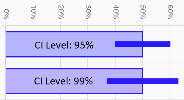
A higher confidence level means that the confidence interval will be larger. As an intuitive example, if you arrive in a new city and only 5 out of 20 people that you've seen so far have been students, it's a good guess that less than half the people in the whole city are students, but would you bet your life on it? Probably not, but you'd probably be okay betting your life that less than 99% are students. In general, if you want to be really confident about a claim, you need to be more vague about what you're claiming.
So what confidence level should you choose? There are no right answers here, just popular ones. 95% is the most common (e.g., if you see poll results on the news with a margin of error of +/- 3%, they're probably using a 95% confidence level). Other common levels are 90%, 98% and 99%. And physicists and engineers shooting for 6 sigma of certainty are using a confidence level above 99.999%.
Sample Size
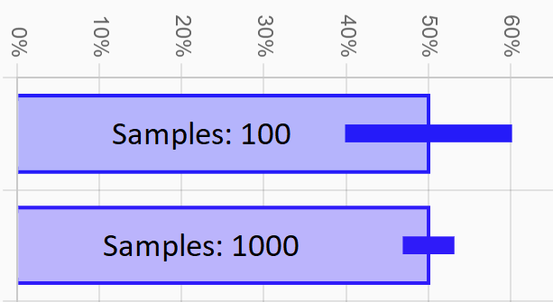
The more data you have, the more confident you can be about the results, which means the larger the sample size, the smaller the CI. For example, if you approach 1 lead and don't get the contact, we can't really say much about your results because we only have a sample size of 1. If instead you approach 1,000 leads and still get no contacts, we can be really confident that you really suck. If you want small CIs with a high level of confidence, you need to increase your sample size.
In more technical terms, the CI size is inversely proportional to the square root of the the sample size. So as a rule of thumb, if you want to shrink you CI to half its size, you need 4 times the number of samples.
Estimated Rate
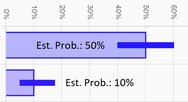
The estimated rate is the rate that we can calculate from the limited data we've collected so far, whereas the true rate is the unknown value we are trying to measure and bound. Think of the true rate as the result we'd achieve if we approached an infinite amount of similar leads.
Obviously the estimated rate of the data you've already collected will affect the position of the CI, but the width of the CI will also shrink as your estimated rate moves closer to 0% or 100%. This is because we are measuring what's called a binomial random variable, which means that each sample can only result in 1 of 2 outcomes (i.e., success or fail). Therefore, if the estimated rate is around 50%, then our samples are maximally varying, meaning we can expect large shifts in our results if we run multiple tests on the same population. Conversely, if the estimated rate is very low or very high, our results are less erratic and we can be more certain about our estimates. More technically speaking, the CI size is proportional to the square root of the probability of success times the probability of failure.
Although this all technically means you can tighten up your CIs by sucking more, we do not recommend this strategy.
How To Use CIs
Confidence intervals are a great tool for identifying which results are actually relevant and which are simply due to random chance. Let's analyze an example situation discussed at the beginning of this section to see how CIs can help:
Let's say you approached 20 leads last week and were able to get 13 contacts. That's a rate of 65%. Then at the start of this week you got a haircut, and afterwards approached 7 leads resulting in only 1 contact. That's a rate of 14%! What happened?! Does your haircut suck that badly or are you just unlucky? Before you freak out and burn down your barber's salon, let's look at your CIs just to be sure.
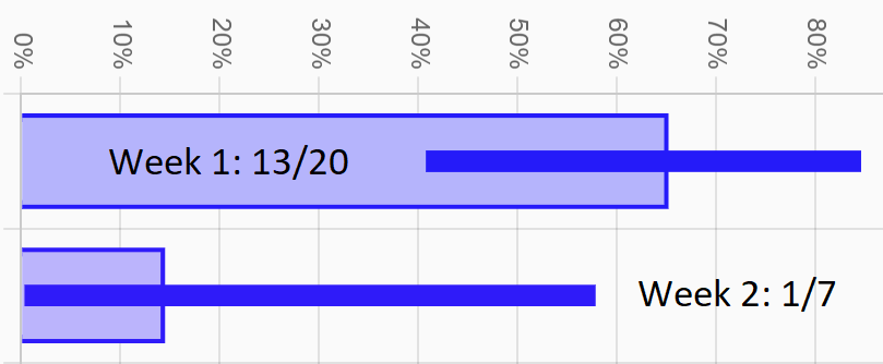
The CI for last week ranges from 41% to 85%, and the CI for this week is 0% to 58%, meaning there's an overlap between 41% and 58%. This means that for our level of confidence (95%), our results so far show that it is entirely possible that our true rate for both weeks was identical and somewhere between 41% and 58%, and our weird results are just due to random chance. In fact, it's even possible that our haircut helped us to push our true rate up from 45% to 55%. This isn't the same as claiming that these alternative explanations are likely. We're only showing that we can't rule them out yet. To get more clarity, we'll need more data.
Determined to find out if you should demand a refund for your haircut, you commit to approaching more leads to get better data. At the end of the week, you've collected 9 contacts from a total of 40 approaches, improving your rate to 23%. Maybe your haircut isn't so bad after all...
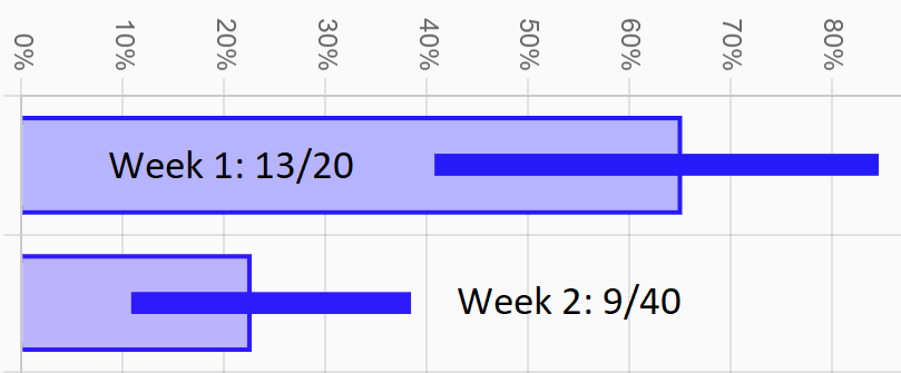
Sunuvabitch! The new CI for this week ranges from 11% to 38%. So we can be confident that you're below 38% this week and you were at least 41% last week, meaning you're confident that random chance isn't the reason for the difference you're observing.
So is it your bad haircut? Maybe. We're confident now it's not just random chance, but it's up to you to figure out what's really going on. Maybe you're overusing your lines and coming off as robotic. Or maybe you look identical to the infamous serial-killer/rapist that just escaped from prison on Sunday.
How NOT To Use CIs
Yes, CIs can be mishandled/misapplied, and one of the most common ways is called p-hacking ("p" refers to the variable p that's usually used to represent the CI level). As Wikipedia describes, p-hacking "is the misuse of data analysis to find patterns in data that can be presented as statistically significant, thus dramatically increasing and understating the risk of false positives. This is done by performing many statistical tests on the data and only reporting those that come back with significant results."
You may be thinking, "Well I don't need to worry about that. Why would I misrepresent my own data to lie to myself?" However, while possible to perform intentionally, p-hacking is so easy to do accidentally that even serious researchers and scientists need to take precautions against it. Here's 2 examples on how you could easily p-hack yourself:
Let's say that you just had a decent month, and you'd like to know if in the future you're ever getting better or worse, so you decide to measure your results each week and see if the CI diverges enough to show a positive or negative change. You set your CI level to 95% because that's what everyone uses. 3 months later you have a week where your CI is fully below the original month's CI, and you start freaking out because you're sure you must be getting worse. Well, the bad news is you're being a dumbass, but the good news is you probably just p-hacked yourself instead of getting worse. Because your CI level was 95%, this means that 1 out of every 20 CI bars is lying to you. So even if you performed identically every week, in about 20 weeks you can expect to see one week (on average) that shows supposedly significant changes.
Even if you're not running formal tests like the previous example, you can still subtly p-hack yourself. Imagine that your looking at your skill chart, which shows 8 skills in total, and you're comparing various filters against your raw unfiltered data to see if the filters make a significant difference. You've also heard of this p-hacking thing, so you set your confidence level up to 98% just to be sure. You look at a few filters without seeing a significant difference and then finally find an interesting result... apparently, approaching leads on a Tuesday night significantly improves your ability to successfully get verbal confirmations on any of the resulting meetings you get from said approaching. Well, maybe, but it's also very possible that you just p-hacked yourself again. Each filter you casually look at contains 8 CIs, and 1 out of 50 of those CIs is wrong, so on average you'll see about 1 incorrect CI for every 6 filters you check against.
If you still don't see the problem, maybe this XKCD comic will make things clearer.
So how can you guard against p-hacking? The easiest way is to use higher CI levels, but then all your CI bars might grow out of control. If you have some self awareness and discipline, just keep in mind that your brain likes to ignore uninteresting results and amplify the interesting ones, so only take the results seriously if you conducted the test seriously too.
Which CI Type Should You Use?
Bayesian.
But What About Those Other CI Types?
Oh, so you don't trust us, huh? You want to know the other options and how they work so you can decide for yourself? We find your lack of faith disturbing.
None
Reality is deterministic. Everything happens for a reason and couldn't have happened any other way. Statistics is for witches and heretics. If you agree with this (or maybe you just don't want to be accidentally p-hacking yourself) then choose this option.
Normal
The other types aren't weird. It's just that this type of CI is based on what's called a "normal distribution". The normal distribution (aka, Gaussian distribution) is the big daddy of all variable probability distributions. In fact according to the "Central Limit Theorem", all random variable probability distributions tend towards the normal distribution if you add enough samples together. And this is exactly the reason why we can use the normal distribution as well. Even though the distribution of any of our given binomial samples (either "success" or "failure") is basically the antithesis of the smooth normal distribution, if we add enough samples together, they eventually take the shape of the normal distribution.
Let's look at a specific example to make things clearer. Imagine we're measuring your ability to get contacts from leads, and you got 50 numbers out of 100 leads. Let's assume that we can represent the properties of the results with a normal distribution, for which we only need to know the mean (\(\mu\)), which tells us the center position and represents the true rate of success, and the standard deviation (\(\sigma\)), which tells us the distribution's width. For a binomial variable we can calculate the standard deviation using the equation below, where \(p\) is the success rate, and \(n\) is the number of samples. The calculation results in a standard deviation of 0.05, and the picture shows the resulting effective distribution (we don't know the true rate of success \(\mu\) yet, but we will place it at 50% for now so we can draw our picture). \[\sigma=\sqrt{\frac{p(1-p)}{n}}\]
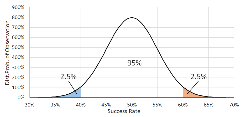
So, what does this normal distribution represent, or any probability distribution for that matter? Well, it shows the probability of a certain value occurring. More specifically for our needs, if we cut out a specific chunk of the curve, the area of what we cut out gives us the probability that the value will be inside that chunk. For example, in the image, the blue and orange sections each contain 2.5% of the area under the curve, with the other 95% in the center. So if we were to sample a random variable with this distribution, 2.5% of the time we'd land in the blue area (less than 40.2% success rate), 2.5% of the time we'd land in the orange (greater than 59.8% success rate), and 95% of the time we'd land somewhere in the middle (success rate between 40.2% and 59.8%). To clarify again, although each sample is a success or failure, if we collect 100 of these samples together, the success rate we observe from that group of samples will take on a value predicted by this normal distribution.
Now, we don't yet know where we should slide the center of this distribution to because we still don't know what the true success rate is. So here's the final trick: if we could guarantee that the resulting mean \(p\) of our previous set of 100 samples fell somewhere in the center 95% of our distribution, what could we then guarantee about the center position of the distribution? Well, if we slide the distribution as far possible to the right (blue curve), we see that we can't go further than \(\mu\) = 59.8%, because going further would imply that our 100-sample result came from the bottom 2.5% of the true distribution. Similarly, as we move the distribution to the left (orange curve, we can't move \(\mu\) lower than 40.2%
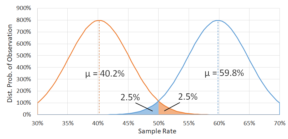
So putting it all together, if we can assume that our sample set results can be approximated by a normal distribution, and we can calculate its standard deviation, and we can guarantee that our result must have come from the center 95% of that distribution, then we can guarantee that the true success rate (assuming we collected an infinite number of samples) would be between 40.2% and 59.8%, which becomes our confidence interval. Now, we can't actually guarantee that our 100-sample run result came from the central 95% of the distribution, but we can be 95% confident that this was the case, so we can also be 95% confident in our new CI.
Disadvantages
Unfortunately, we made several bold assumptions in our explanation that don't always hold true and can seriously affect our CI:
- We can move the distribution around without affecting its shape - Moving the distribution center means we're changing its average value, but we already showed how the standard deviation (and therefore the distribution width) is dependent on the average value. We just ignored this inconvenient fact because it complicated our analysis.
- We can always calculate the standard deviation - What happens when out of 5 leads you have all failures or all successes? Well, your computed standard deviation goes to 0, which seems to 100% guarantee that you will continue to get 100% failures or successes forever. That's obviously nonsense, which means our method/assumptions aren't working in this special case.
- We can approximate our results with a normal distribution - "But weren't you just sayi-" Yes, we know what we said, but this isn't always a good assumption to make, especially if there were a low number of successes or failures. In these cases the actual distribution becomes lopsided. It also makes no sense that the normal distribution would be so smooth if we're running tests on a small sample size. You can't have 11.3 successes.
Who Should Use It?
People that prefer simplicity over accuracy and rationality. We mostly included it because it's popular.
Exact
The Exact CI (more formally referred to as the Clopper–Pearson CI) is so called because it uses the exact distribution for describing binomial distributions instead of using some basic normal approximation that results in all kinds of weird issues. Here's the equation for the binomial distribution in all its glory:\[\mathrm{P}(X=k)=\binom{n}{k}p^k(1-p)^{n-k}\]
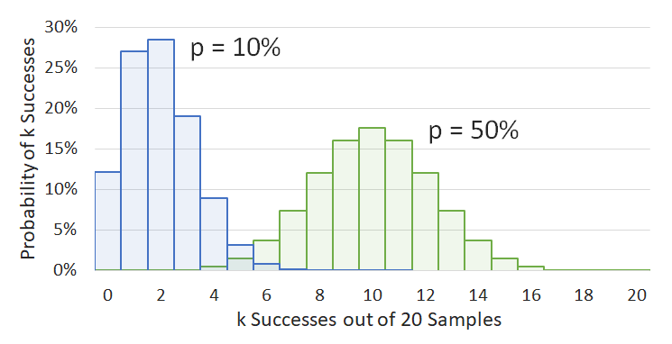
Okay, that looks complicated, but it's not actually that bad. It just tells us what the probability is of observing \(k\) successes if we have \(n\) samples and the true rate of success is \(p\). As an example, we have an image showing 2 different probability distributions. Both distributions show the probability of observing \(k\) results out of 20 samples, with the left blue graph showing what would happen if the true success rate were 10%, and the the right green graph showing the same but for 50%. Notice how the binomial distribution is different from the normal distribution: it is lopsided when it approaches the edges, and it is discrete instead of continuous (it doesn't make sense to consider fractions of a success).
So how do we use the binomial distribution to determine our CI? Well, the general process is almost identical to the process for finding the Normal CI (the math is way harder, but we'll handle that behind the scenes on our end). We'll use another example to demonstrate:
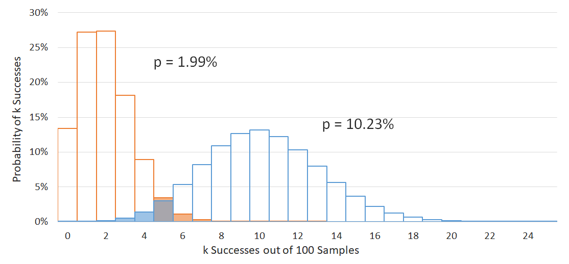
Assume you just approached 100 leads and only collected 5 contacts. Ouch. We're going to look at a 90% CI level this time (makes the graph easier to read), so let's assume that your results come from the central 90% of the true underlying probability distribution we are trying to measure. To get our CI, we just need to adjust our hypothesis about the true success rate \(p\) until the success count \(k\) = 5 falls outside of the central 90% into one of the side 5% regions. As the image below shows, this occurs below \(p\) = 1.99% and above \(p\) = 10.23%, giving us our CI.
Disadvantages
The Exact CI doesn't have many disadvantages. It's a pretty solid tool. If we had to nitpick though, the only real issue is that it's a little more conservative than some other options out there. This means that while it never gives a smaller CI than appropriate, it can sometimes give a CI that's larger than it needs to be.
As an extreme example of this, if you fail at something 5 out of 5 times, a reasonable person wouldn't say with any confidence that what your attempting might be impossible. However, the Exact CI will include 0% no matter what level of confidence you choose, implying that it's plausible that something is impossible simply because it couldn't be done after 5 attempts. Again, this is not to say that the Exact CI is wrong to include 0% in it's CI, but this might convince some people that it's overly conservative in some scenarios.
Who Should Use It?
It's a toss-up between the Exact CI and the Bayesian CI. We recommend both, but prefer Bayesian. Use whichever one feels more intuitive to you.
Bayesian
There are 2 competing schools of thought when it comes to statistics: Frequentist and Bayesian. The Normal CI and Exact CI are Frequentist methods. In short, Frequentist statistics performs all of the analysis with the results of the observed experiment, whereas Bayesian statistics assumes that prior information is important and should affect the analysis. Let's consider a quick example to demonstrate the importance of prior information in Bayesian reasoning:
Imagine there's a new super-COVID out. About 1% of the population has it. It's 100% deadly, but you still want to go see your girlfriend tonight. You don't have any symptoms, but she makes you get tested anyways. At the clinic, the doctor tells you the test is very accurate, giving the correct diagnosis 95% of the time. You take the test. Result comes back positive. Oh shit. You call your girlfriend with the bad news. She cries, "Oh no! This is terrible. The test is right 95% of the time. That's a high level of confidence". Then she calms down and says, "I guess I'll have to find a new man" -- "Wait you dumb Frequentist!" you exclaim. "You haven't considered the prior probabilities!"
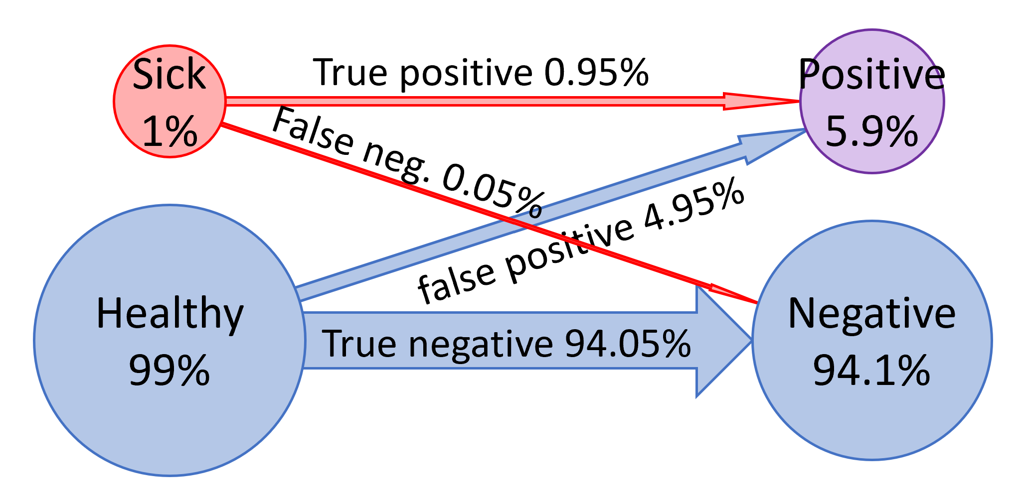
Let's take a step back and pretend we hadn't just gotten tested? What's the likelihood that we would test positive? We need to consider all possible paths that lead to you testing positive and sum them together. First, there's the chance you were sick (1%) and then the test worked (95%), meaning this reality has a 0.95% chance of occurring. Second, there's the chance that you weren't sick (99%) but the test failed (5%) giving a positive result anyways, resulting in a 4.95% chance of this reality occurring. Adding these 2 possibilities together produces a total probability of 5.9% that you would test positive regardless of whether you were actually sick or not. Now, let's consider again that we now know for a fact that you did test positive. That little 5.9% of possibility has blown up to 100% of our reality. So how did we get here? Well we can just divide our original options by 5.9% to find out. Turns out there's only a 16.1% chance we were sick in the first place and an 83.9% chance that the stupid test is a liar!
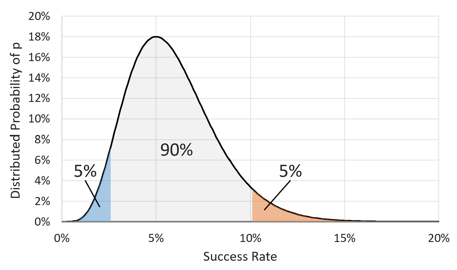
Following the general example above, we can apply the same type of analysis to the binomial distribution to work backwards from our observed reality and find our most likely original state, by which we mean the state of \(p\), our true underlying success rate. Unfortunately, unlike in the previous example, we have no a priori knowledge about which values for \(p\) are most likely, so we will assume that all values from 0% to 100% are equally likely. Let's also assume, as with the Exact CI discussion, that you've just collected only 5 contacts out of your last 100 leads. Now that we've observed our final circumstances (5 successes out of 100), how likely is it that we got here from any possible value of \(p\)? In the super-COVID example, there were only 2 original states that we needed to consider, but now there's a whole spectrum of possible values for \(p\), so we've just graphed the results on the chart.
It may be hard to tell, but the area under the curve is equal to 0.99%. However, as with the 5.9% chance to test positive in the super-COVID example, we don't necessarily care how likely we were to get 5 out of 100 successes. We only care about the relative probabilities of how we got here. And now that we can see what those relative probabilities are in the graph, we simply take the central 90% of the area under the curve and call it a day. So for our example, the 90% confidence interval is from 2.62% to 10.13%. Actually, in Bayesian statistics it's called a certainty interval, but we'll just call them both CIs anyways.
Disadvantages
None that we're aware of, but it's not as popular, and your frequentist buddies may object.
Who Should Use It?
We prefer the Bayesian CI because it seems more intuitive than the Exact CI, but you do you.
And if you still need more help deciding between Exact or Bayesian, this XKCD comic might shed some light.